
A (Practical) Framework for Quantifying Cyber Risk: Part 1
Introduction
In this series, I will summarize my journey into risk quantification using FAIR, a mathematically and statistically sound framework for quantifying cyber risk, which should help infosec practitioners move beyond traditional qualitative assessments (read: the usual Risk Heath Map) to a more sound (and defensible) financial approach.
Why Quantifying Risks?
Picture these two situations:
Two CISOs are asking the board of directors to approve a budget for a new firewall:
CISO #1: “Our current perimeter solution lacks support for deep packet inspection, behaviour-based heuristics, and automated threat intelligence feeds. Without advanced Layer 7 filtering and real-time AI-based anomaly detection, we can’t fully leverage zero-trust architectures or mitigate zero-day exploits leveraged by state-sponsored actors.”
CISO #2: “Currently, phishing is our top threat vector, exposing us to potential regulatory fines and loss of customer trust. We’re requesting €300,000 to implement advanced email filtering and encryption. Our quantitative risk analysis indicates that a major breach could result in losses and fines of up to €10 million. This investment is projected to cut that risk by 80%, yielding an 8:1 return in value protection and compliance assurance.”
Which of the two CISOs is more likely to obtain the funding? This is why you need to know FAIR.
At the end of this article, you should be able to understand why it is essential to quantify risks and how FAIR can be used to express a risk in financial terms, which will facilitate better communication with business leaders.
The Problem with Heat Maps
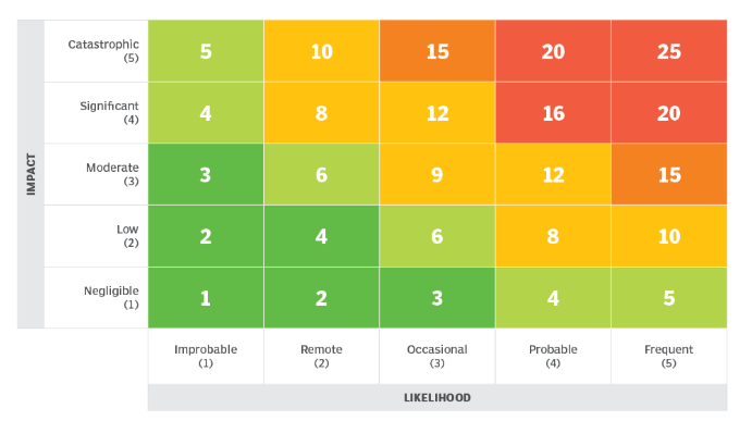
A Typical 5×5 Heatmap (Source: Techtarget)
Risk heat maps are no longer cutting it these days. Here is a summary of the most significant issues they introduce:
They oversimplify complex risks, condensing nuanced risk factors into basic color-coded categories (e.g., red, yellow, green), which can lead to loss of critical detail and nuance.
Risk heat maps heavily rely on subjective scoring for likelihood and impact, resulting in inconsistency and potential bias across assessments.
These visual tools provide a false sense of precision, as arbitrary numerical ratings may give an illusion of accuracy that doesn’t reflect reality.
Heat maps fail to account for risk dependencies and interactions between risk scenarios, resulting in a poor understanding of how risks may compound or evolve together.
The methodology offers weak support for business decisions, as it cannot easily answer how much a risk might cost, whether mitigation is worth the investment, or provide a clear ROI for risk-reduction strategies.
The FAIR Framework
The primary methodology leveraged here is the FAIR (Factor Analysis of Information Risk model. FAIR aims to solve the limitations of traditional, qualitative risk assessment methods by enabling organizations to quantify information and cyber risks in clear financial terms. It provides a structured, quantitative approach that supports objective, data-driven decision-making and better aligns risk management with business priorities and resource allocation.
The beauty of this methodology is that you can delve as deeply as needed, depending on the criticality of the risk being examined. For example, you could supplement your analysis with a Monte Carlo simulation to account for uncertainty and generate a distribution of potential financial losses for critical risks. Still, you could just use educated guesses for less critical risks. It will still be better than a heat map!
The FAIR framework provides a robust and defensible methodology for quantifying cyber risk in financial terms. By combining the structured ontology of the FAIR model with the probabilistic power of Monte Carlo simulations, organizations can gain a much deeper and more actionable understanding of their cyber risk posture. This enables a shift from a compliance-driven to a risk-driven security strategy, where investments are prioritized to mitigate the most significant financial loss exposures.
Components and Formulas
In its essence, the FAIR model is a structured ontology that breaks down risk into its fundamental components. The core formula for risk is:
Risk = LEF × LM
The formula calculates the probable financial loss over a given period, typically expressed as Annualized Loss Expectancy (ALE). Let’s examine the factors in more details.
Loss Event Frequency (LEF)
Think of Loss Event Frequency (LEF) as the probability for something bad to happen within a given time frame (typically one year). It is calculated by multiplying two factors:
LEF = TEF × Vuln
Let's explore these terms in more detail.
Threat Event Frequency (TEF) is the probable frequency, within a given timeframe, that a threat agent (i.e., a bad guy) will act against an asset.
This can be further broken down into (but feel free to skip over this, as it is not essential for most risks you will analyze):
Contact Frequency (CF): How often a threat agent is likely to come into contact with an asset.
Probability of Action (PoA): The likelihood that a threat agent will act against the asset once contact has occurred.
Vulnerability (Vuln) is simply the probability that a threat event will become a loss event (i.e., one that will impact your business).
Once again, this can also be analyzed further based on the threat’s capability and the asset’s resistance strength (again, feel free to skip over this as it is only important in some edge cases)
Threat Capability (TCap): The level of force/skill a threat agent can apply.
Resistance Strength (RS): The strength of the control measures in place to resist the threat.
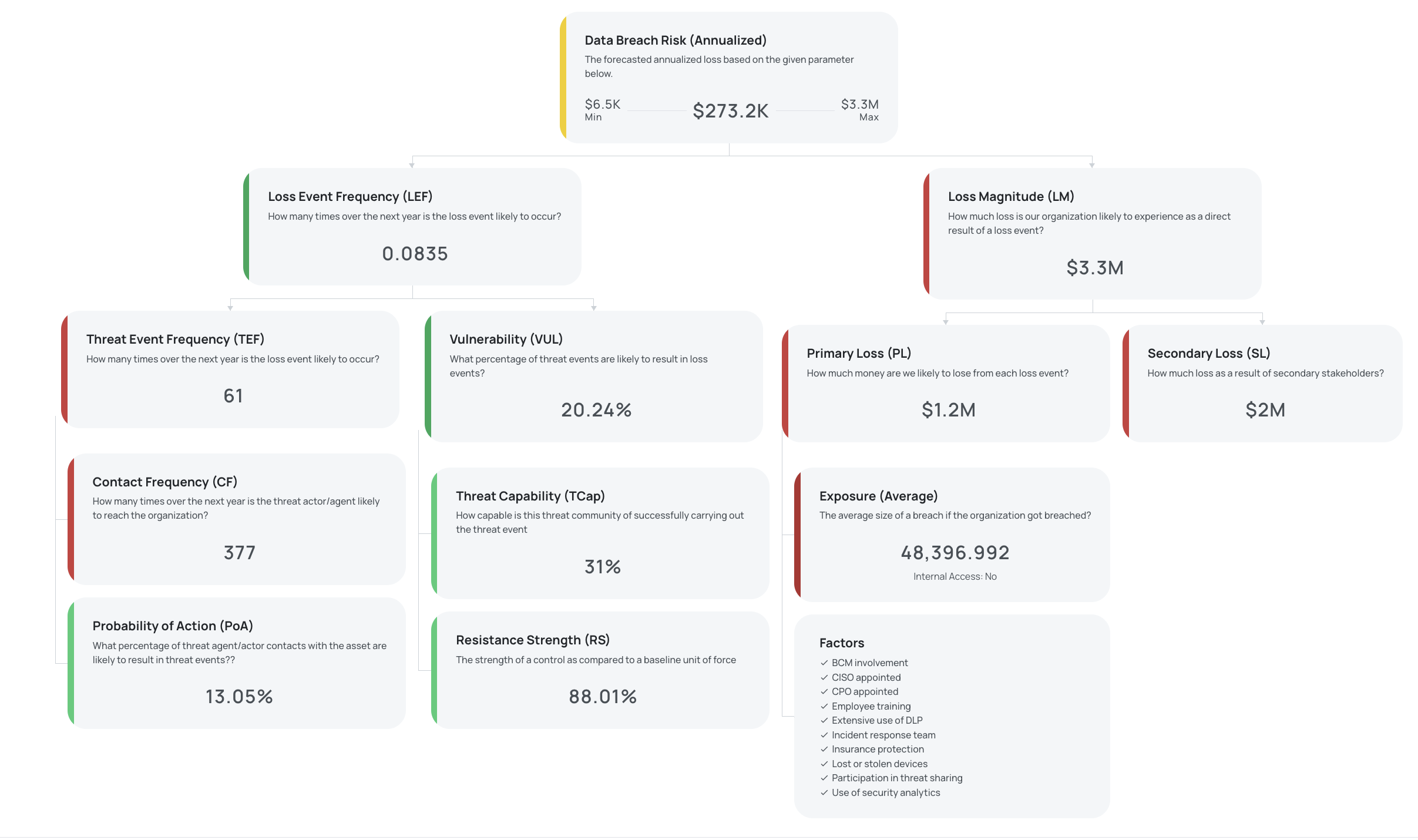
An example of a risk quantification using FAIR (Source: Black Kite)
Loss Magnitude (LM)
The Loss Magnitude (LM) represents the probable financial impact of a single loss event, and it is composed of two forms of loss:
Primary Loss (PLM): The direct financial losses resulting from the event itself. This includes, for example:
Productivity Loss: Reduced or lost revenue, cost of idle employees.
Response Costs: Incident response, forensics, legal fees, and other related expenses.
Replacement Costs: Cost to repair or replace the affected asset.
Secondary Loss (SLM): The indirect financial losses that arise from the reactions of external stakeholders. This includes:
Fines and Judgements: Regulatory penalties and legal settlements.
Reputation Damage: Customer churn, increased capital costs, etc.
Competitive Advantage: Loss of market share or intellectual property.
SLM might also have its own frequency (i.e., it might occur only x out of y times), which is referred to as Secondary Loss Event Frequency (SLEF). Again, feel free to disregard this as, similarly to other sub-definitions, it might be important only in some edge cases. What you need to remember here is that certain risks may be associated with secondary losses — a typical example is a class lawsuit or a fine from the regulator resulting from data breaches.
The Importance of Data Quality
As the old saying goes, “garbage in, garbage out.” Thus, the accuracy of a quantitative risk model is highly dependent on the quality of the input data. The data you need can be sourced from a variety of places:
Threat Event Frequency (TEF)
Internal incident logs and security monitoring tools (SIEM, IDS/IPS)
Threat intelligence feeds and reports
Industry data sharing groups (ISACs)
Publicly available breach data (e.g., Verizon DBIR, Advisen)
Subject Matter Expert (SME) estimates
Vulnerability (Vuln)
Penetration testing and red team exercise results
Vulnerability scan reports
Control assessment results (e.g., from NIST CSF, ISO 27001 audits)
Configuration management databases (CMDB)
SME estimates on control effectiveness
Loss Magnitude (LM)
Financial statements and asset valuation records
Business Impact Analysis (BIA) reports
Legal and compliance department estimates for fines and judgements
Public relations and marketing estimates for reputational damage
Historical incident cost data (internal and external)
Cyber insurance industry reports
Now that we understand the basics, the next article will guide us through the process step by step.
Until then!